TL;DR
Monte Carlo simulation reshuffles your historical trades thousands of times to reveal the full range of possible outcomes, including worst-case drawdowns that a single backtest cannot show.
Table of Contents
Monte Carlo simulation is a statistical technique that uses repeated random sampling to model the probability distribution of possible outcomes. Named after the famous Monte Carlo Casino in Monaco, the method was originally developed during the Manhattan Project in the 1940s by scientists Stanislaw Ulam and John von Neumann. In trading, Monte Carlo simulation takes a set of historical trade results and randomly reorders them thousands of times to generate a distribution of possible equity curves. Each reshuffling produces a different path because the sequence of wins and losses changes, even though the individual trade results remain the same. By analyzing all of these simulated equity curves, traders can understand the full range of potential outcomes their strategy might produce, including best-case, worst-case, and median scenarios. This is fundamentally different from a single backtest, which shows only one specific sequence of trades that happened to occur in the past.
The process begins with a set of trade results, either from a backtest or from live trading history. The simulation engine then performs the following steps repeatedly. First, it takes all of the trade results and randomly shuffles their order. Second, it calculates the equity curve that would result from that specific sequence of trades. Third, it records key metrics from that equity curve, such as maximum drawdown, final equity, and peak equity. This process is repeated thousands of times, typically between 1,000 and 10,000 iterations. After all iterations are complete, the results are aggregated into probability distributions. For example, you might learn that there is a 95% probability that your maximum drawdown will stay below 25%, or that your median ending equity after 200 trades is $18,500. The power of Monte Carlo simulation lies in the law of large numbers: with enough iterations, the distribution of outcomes converges to the true probability distribution of your strategy's potential performance.
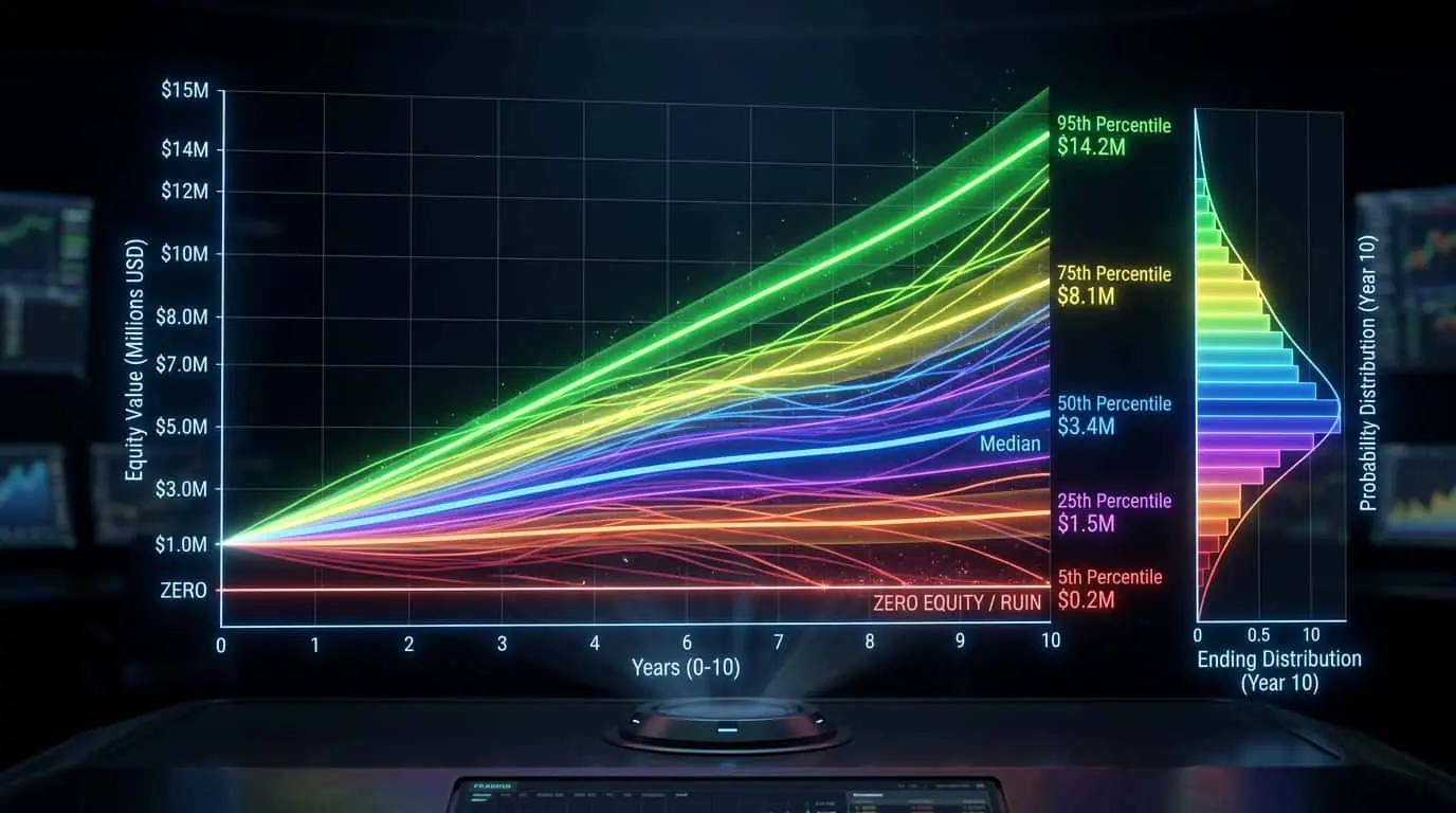
A Monte Carlo simulation produces several critical metrics that go far beyond what a standard backtest provides. The most important is the drawdown distribution, which shows the probability of experiencing various levels of drawdown. While your backtest might show a 12% maximum drawdown, Monte Carlo analysis might reveal a 20% probability of drawdowns exceeding 20% with the same set of trades in a different order. The final equity distribution shows the range of possible ending account values, from the worst-case 5th percentile to the best-case 95th percentile. The risk of ruin probability tells you how likely your strategy is to hit a catastrophic drawdown level, such as 50% or more. These metrics are essential for setting realistic expectations and making informed decisions about position sizing and capital allocation.
| Metric | What It Shows | Why It Matters |
|---|---|---|
| Median Final Equity | The middle outcome across all simulations | Most realistic expectation of strategy performance |
| 5th Percentile Drawdown | Worst-case drawdown at 95% confidence | Determines if strategy can survive bad luck |
| Risk of Ruin | Probability of hitting a catastrophic loss level | Decides whether strategy is safe to trade at all |
| 95th Percentile Equity | Best-case outcome at 95% confidence | Shows upside potential under favorable conditions |
| Sharpe Ratio Distribution | Range of risk-adjusted returns | Evaluates consistency across different scenarios |
A standard backtest runs your strategy through historical data in chronological order and produces a single equity curve with a single set of performance metrics. This is useful but inherently limited because it represents only one possible path out of millions. The specific sequence of wins and losses in the historical data may never repeat. A strategy that had a smooth equity curve in a backtest might have experienced a devastating drawdown if just a few trades had occurred in a different order. Monte Carlo simulation addresses this limitation by exploring thousands of alternative sequences. It answers the question: given these trade results, what is the full range of possible outcomes? This makes it a stress test for your strategy. If your strategy shows a 15% maximum drawdown in a backtest but Monte Carlo analysis reveals a 30% drawdown at the 95th percentile, you know the backtest was optimistic. Conversely, if Monte Carlo confirms that drawdowns stay manageable across most simulations, you can trade with greater confidence.
Pro Tip
Run Monte Carlo simulation on at least 100 trades for statistically meaningful results. With fewer trades, the distributions are too wide to draw reliable conclusions. Aim for 200+ trades and 5,000+ iterations for robust analysis.
Monte Carlo simulation has several direct applications in real-world trading. The first and most common is position sizing validation. If your Monte Carlo analysis shows that a 2% risk per trade could lead to a 40% drawdown at the 95th percentile, you might reduce your risk to 1% per trade to keep worst-case drawdowns within acceptable limits. The second application is prop firm evaluation: if a prop firm allows a maximum 10% drawdown, Monte Carlo analysis tells you the probability of violating that rule with your strategy. The third application is comparing strategies. Two strategies with similar backtest results might show very different Monte Carlo distributions, revealing that one is more robust than the other. Finally, Monte Carlo simulation helps set realistic profit expectations. Instead of assuming your backtest return will repeat, you can plan around the median or even the 25th percentile outcome for conservative financial planning.
Understanding the mathematical foundation of Monte Carlo simulation helps traders interpret results correctly. The core concept is building an empirical probability distribution from resampled data. Suppose your strategy produced 200 trades with a mean profit of $150 and a standard deviation of $400. A single backtest yields one equity curve, but Monte Carlo generates thousands of curves by randomly sampling with replacement from those 200 trades. After 5,000 iterations, you can rank all 5,000 final equity values from lowest to highest. The 250th value (5th percentile) gives you the worst-case outcome at 95% confidence. The 2,500th value (50th percentile) is the median. For drawdowns, the same ranking applies: sort all 5,000 maximum drawdowns and read off the percentile you need. For example, if your backtest showed a $10,000 final profit and a 15% maximum drawdown, Monte Carlo might reveal the following distribution: at the 5th percentile, final equity could be as low as $3,200 with a drawdown of 28%; at the 50th percentile, $9,500 with a 19% drawdown; and at the 95th percentile, $16,800 with only a 10% drawdown. The width of these distributions depends on the consistency of your trades. A strategy with a high Sharpe ratio (low standard deviation relative to mean) will produce tight distributions, meaning outcomes are predictable. A strategy with a low Sharpe ratio will produce wide distributions, meaning outcomes vary drastically based on trade order.
Confidence Percentile = Iteration_Rank / Total_Iterations x 100Iteration_Rank — Position when all outcomes are sorted ascending
Total_Iterations — Total number of Monte Carlo simulations run
| Percentile | Meaning | Example (200 trades, $150 avg profit) |
|---|---|---|
| 5th | Worst case at 95% confidence | Final equity $3,200, max DD 28% |
| 25th | Conservative planning scenario | Final equity $6,800, max DD 22% |
| 50th (Median) | Most likely outcome | Final equity $9,500, max DD 19% |
| 75th | Favorable scenario | Final equity $12,100, max DD 14% |
| 95th | Best case at 95% confidence | Final equity $16,800, max DD 10% |
While NinjaTrader 8 does not include a built-in Monte Carlo simulator, you can integrate Monte Carlo analysis into your NinjaTrader workflow effectively. After running a backtest in NinjaTrader's Strategy Analyzer, export the trade list to CSV. This export includes entry time, exit time, profit/loss, and other trade details. You can then import this data into a Monte Carlo tool (such as our free Monte Carlo Simulator) to generate probability distributions. The process takes about 60 seconds once you have your trade export ready. When evaluating your NinjaTrader strategy results, pay special attention to the distribution shape. If your strategy relies on a few large winners (a common trait in trend-following NinjaScript strategies), Monte Carlo analysis may show wide equity curve distributions because those big winners could appear at different points in the sequence. Strategies with more consistent, smaller wins tend to show tighter distributions and more predictable real-world performance. A practical tip for NinjaTrader users is to run Monte Carlo separately on different market conditions: extract trades from trending periods and ranging periods independently. This reveals whether your strategy's robustness depends on market regime, something a single full-sample Monte Carlo cannot show. Also consider running Monte Carlo on your walk-forward optimization results rather than a single in-sample backtest, as this provides a much more realistic input dataset.
Pro Tip
In NinjaTrader, export your Strategy Analyzer trade list via right-click then Export. Run Monte Carlo on the exported trades and compare the 5th-percentile drawdown against your prop firm's maximum drawdown rule or your personal risk tolerance. If the 5th-percentile drawdown exceeds your limit, reduce your per-trade risk until it fits within bounds.
While Monte Carlo simulation is a powerful tool, it has important limitations that traders should understand. The most fundamental is that it assumes trades are independent, meaning each trade's outcome does not affect the next. In reality, market conditions change, and strategies may perform differently in trending versus ranging markets. Monte Carlo simulation also cannot account for regime changes, black swan events, or structural shifts in market behavior. It works with the trade results you provide, so if your backtest is curve-fitted or based on insufficient data, the Monte Carlo results will be misleading as well. Another limitation is that standard Monte Carlo simulation does not model changing position sizes, margin requirements, or the psychological impact of drawdowns. Despite these limitations, Monte Carlo remains one of the most valuable tools available for strategy evaluation, provided traders understand it as one component of a comprehensive analysis rather than a crystal ball.
Mistake
Using Monte Carlo results from a curve-fitted backtest
Correction
Ensure your backtest trades are based on out-of-sample data or walk-forward analysis. Monte Carlo amplifies the reliability of the input data, so garbage in means garbage out.
Mistake
Running Monte Carlo with fewer than 50 trades
Correction
Build a larger sample size through extended backtesting or paper trading. With too few trades, the probability distributions are too wide to draw actionable conclusions.
Mistake
Ignoring the 95th percentile drawdown and focusing only on the median
Correction
Always plan for worst-case scenarios. Size your positions so that even the 95th percentile drawdown is survivable both financially and psychologically.