TL;DR
Correlation measures the statistical relationship between two assets' price movements. Positive correlation (+1) means they move together, negative correlation (-1) means they move oppositely, and zero correlation means no relationship. Understanding correlation is essential for diversification, avoiding hidden concentration risk, and managing portfolio-level exposure.
Correlation is a statistical measure that describes the degree to which two assets' prices move in relation to each other. Expressed as a coefficient ranging from -1.0 to +1.0, correlation quantifies both the direction and strength of the relationship between two price series. A correlation of +1.0 means the two assets move perfectly in lockstep: when one rises 1%, the other rises 1%. A correlation of -1.0 means they move perfectly opposite: when one rises 1%, the other falls 1%. A correlation of 0.0 means there is no linear relationship between their movements. In practice, perfect correlations of +1.0 or -1.0 are extremely rare. Most asset pairs fall somewhere in between, and the correlation itself fluctuates over time based on changing market conditions, economic regimes, and investor behavior. For traders, correlation is not just an academic concept -- it is a critical risk management tool. If you hold simultaneous positions in two highly correlated instruments, you effectively have double the exposure to a single risk factor, even though it may appear you are diversified across two different markets. Understanding correlation reveals hidden concentration risk, helps optimize position sizing across multiple instruments, and enables hedging strategies that reduce overall portfolio volatility.
Positive correlation occurs when two assets tend to move in the same direction. The strength of the positive relationship determines how reliably they move together. Strong positive correlation (0.70 to 1.00) means the assets move together most of the time, driven by shared underlying factors. The ES (S&P 500) and NQ (Nasdaq) futures have a historically strong positive correlation, typically between 0.85 and 0.95, because both are US equity indices with significant overlap in constituent companies. Gold mining stocks (GDX) and gold futures (GC) also show strong positive correlation, typically 0.75-0.90. Negative correlation occurs when two assets tend to move in opposite directions. The classic example is the historical relationship between US Treasury bonds (ZN, ZB) and the S&P 500: during risk-off events, money flows out of stocks and into the perceived safety of government bonds, creating an inverse relationship. This correlation has typically been -0.20 to -0.50 over the past two decades, though it can shift during unusual monetary policy regimes. The US dollar index (DX) and gold futures (GC) also tend to show negative correlation, because gold is priced in dollars and becomes relatively cheaper for foreign buyers when the dollar weakens. Zero or low correlation means no reliable directional relationship exists. Crude oil (CL) and corn futures have near-zero correlation during most periods because they are driven by fundamentally different supply and demand dynamics -- one by global energy markets, the other by agricultural conditions.
| Asset Pair | Typical Correlation | Relationship | Driving Factor |
|---|---|---|---|
| ES (S&P 500) / NQ (Nasdaq) | +0.85 to +0.95 | Strong positive | Both are US equity indices with overlapping stocks |
| Gold (GC) / Silver (SI) | +0.75 to +0.90 | Strong positive | Both are precious metals driven by similar macro factors |
| EUR/USD / GBP/USD | +0.70 to +0.85 | Strong positive | Both primarily reflect USD strength or weakness |
| S&P 500 / US Treasuries | -0.20 to -0.50 | Moderate negative | Risk-on/risk-off capital flow between stocks and bonds |
| USD Index / Gold | -0.30 to -0.60 | Moderate negative | Gold priced in USD; weak dollar supports gold prices |
| EUR/USD / USD/CHF | -0.85 to -0.95 | Strong negative | Both pairs are USD-driven but on opposite sides |
The primary practical application of correlation for most traders is portfolio diversification -- structuring a portfolio so that losses in one position are offset or reduced by gains in another. True diversification requires holding assets with low or negative correlation. A portfolio of ES, NQ, and RTY (Russell 2000) is not truly diversified because all three are US equity indices with high positive correlation. A portfolio of ES, ZN (10-Year Treasuries), GC (Gold), and CL (Crude Oil) is far more diversified because these assets respond to different economic factors with low or mixed correlations. The mathematical benefit of diversification is significant. If two assets each have 20% annual volatility and zero correlation, a 50/50 portfolio has approximately 14.1% volatility (20% divided by the square root of 2), not 20%. The portfolio volatility is lower than either individual asset because their movements partially cancel out. With negative correlation, the reduction is even greater. For systematic traders who run multiple strategies, correlation analysis is essential. If Strategy A and Strategy B both perform well in backtesting, the combined value depends heavily on their correlation. Two strategies with a correlation of 0.90 provide almost no diversification benefit -- you might as well run either one at full size. Two strategies with zero or negative correlation produce a combined equity curve that is significantly smoother than either strategy alone, reducing maximum drawdown and improving the Sharpe ratio.
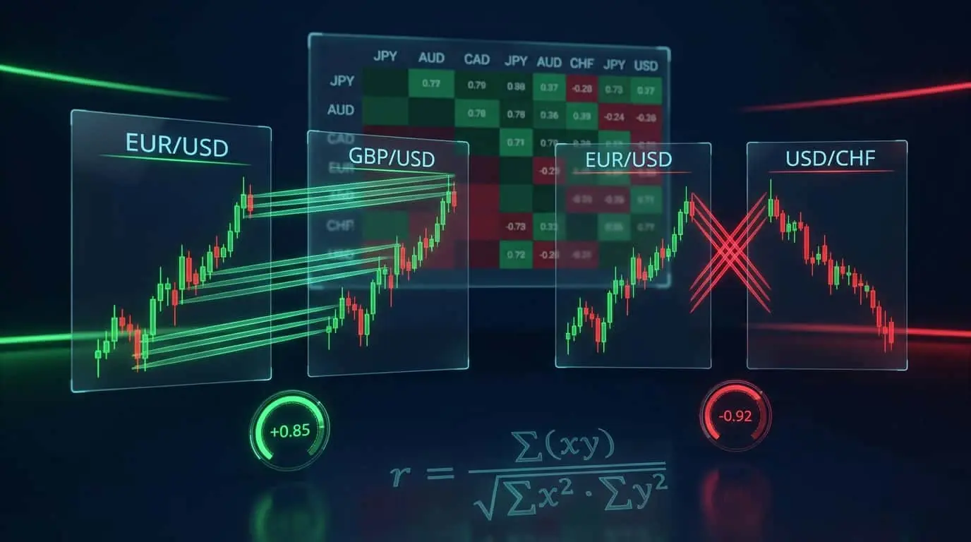
r = Sum[(Xi - X_mean)(Yi - Y_mean)] / sqrt(Sum[(Xi - X_mean)^2] * Sum[(Yi - Y_mean)^2])r — Pearson correlation coefficient, ranging from -1.0 to +1.0
Xi, Yi — Individual returns of asset X and asset Y for each period
X_mean, Y_mean — Mean (average) returns of each asset over the sample
One of the most important and often overlooked aspects of correlation is that it changes over time, sometimes dramatically. Correlations that hold during normal market conditions can break down or even reverse during market stress, precisely when you need diversification the most. This phenomenon is called 'correlation breakdown' or 'crisis correlation.' During the 2008 financial crisis, correlations between asset classes that were historically uncorrelated (or negatively correlated) spiked toward +1.0 as a global flight to cash caused simultaneous selling across nearly all risky assets. Stocks, commodities, corporate bonds, emerging markets, and even some traditionally safe-haven assets all declined together. The only asset class that maintained its negative correlation with stocks was US Treasuries. The practical implication is that you cannot simply calculate a correlation once and assume it will hold indefinitely. Rolling correlation -- calculating the correlation over a moving window (e.g., the trailing 60 days) -- reveals how the relationship is evolving in real-time. If the rolling correlation between your portfolio positions is increasing, your effective risk exposure is growing even if your nominal positions have not changed. Regime-dependent correlation analysis takes this further by calculating correlations separately during bull markets, bear markets, and high-volatility environments. You may find that two assets have near-zero correlation during calm markets but correlations above 0.80 during sell-offs. This means your diversification works during the easy times but fails during the hard times, which is the worst possible outcome.
Implementing correlation analysis in your trading does not require a statistics degree. Several practical tools and approaches make it accessible. Our correlation calculator allows you to input two assets and a time period to compute the Pearson correlation coefficient and visualize the relationship. Use it to check correlations before adding new positions to your portfolio. For daily monitoring, create a correlation matrix that shows the pairwise correlation between every instrument you trade. Update this weekly or monthly. At a glance, you can identify which positions are providing true diversification and which are redundant. A simple correlation-adjusted risk framework works as follows: define your total portfolio risk budget (e.g., 5% of account equity at risk across all positions). For positions with correlation below 0.30, count them as independent risks. For positions with correlation between 0.30 and 0.70, count each additional position as 0.5 of a full risk unit. For positions with correlation above 0.70, count them as the same risk unit. This ensures that your total portfolio risk does not accidentally exceed your budget due to hidden correlation. For pairs trading and spread trading, correlation is the foundation. Pairs traders look for assets with high historical correlation that have temporarily diverged, betting that the relationship will revert to its mean. This requires monitoring both the absolute correlation and the current spread between the two assets relative to its historical range.
Pro Tip
Check correlations at least monthly, and always after major market regime shifts (central bank policy changes, geopolitical events, sector rotations). Correlations that were valid three months ago may not hold today.
Mistake
Assuming you are diversified because you hold multiple instruments
Correction
Check the correlation between every pair of positions. ES, NQ, and RTY are all US equities with 0.85+ correlation. That is one bet, not three. True diversification requires adding assets with low or negative correlation.
Mistake
Relying on historical correlation without monitoring for changes
Correction
Use rolling correlation (60-day window) and update your analysis monthly. Correlations shift with market regimes, and a diversification strategy based on outdated correlations provides false security.
Mistake
Ignoring correlation when sizing multiple positions
Correction
If you hold two positions with 0.90 correlation, your effective portfolio risk is nearly double what each position suggests. Reduce individual position sizes or treat correlated positions as a single risk unit in your daily loss budget.